As with other disciplines, physical oceanographic characterization requires a suite of complementary technologies that allow researchers to observe the multiple facets that comprise the entire water column to understand the complexities of the physical environment of Long Island Sound. This means not only measuring three key elements of temperature, salinity and current, but also measuring them over different locations and time frames to capture the four dimensional nature of the dynamic environment that strongly influences the other components of the habitats of the Sound.
Conductivity, Temperature and Depth (CTD)
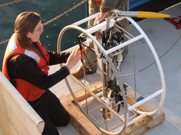
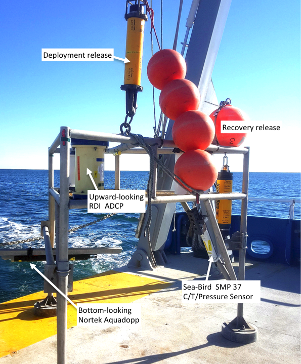
A CTD is a common and essential tool for physical oceanographers and has multiple modes of deployment, as was used by the LIS Seafloor Habitat Mapping Initiative team. A CTD is a collection of sensors bundled into a housing that can be deployed from a ship on its own, or mounted on frame that is deployed along with other sensors and water collectors – both of which are lowered through the water column and recovered to provide a profile of the changes in the measured variables with depth. The CTD can also be mounted on fixed frames that are deployed to the seafloor to record changes in the variables from one site over a period of time, often weeks or months. A CTD can also be mounted on mobile underwater platforms such as a remotely operated vehicle or autonomous underwater vehicle.
The “C” refers to conductivity, ie the ability of water to conduct electricity, which is directly related to the amount of salts dissolved in the water, ie more salts equals greater conductivity. This is then used to calculate the salinity of the water. The “T” refers to temperature that is measured with a simple temperature probe. The “D” refers to depth that is measured by a pressure sensor, which is related to water density and compressibility, with pressure at the surface equal to zero decibars and increasing by one decibar for each meter of depth.
Acoustic Doppler Current Profiler (ADCP)
Scientists have recognized the ability of sound to pass through water and be reflected by various surfaces – this includes tiny particles suspended in the water. They also recognized another property of sound known as the Doppler Effect that occurs when sound reflects off from a moving object – raising the frequency of the reflected sound when the object is headed towards the listener/sensor and lowering as the object moves away. This phenomenon is perhaps best exemplified by the sound of an approaching train or vehicle. This change in frequency, or Doppler Shift, forms the basis for the functioning of an Acoustic Doppler Current Profiler (ADCP), a device used to measure ocean currents. The ADCP sends out acoustic pings at a regular rate at a certain frequency and when the sound reflects from particles moving over the device it undergoes a frequency shift depending upon the direction the particle is heading. The ADCP measures this frequency change to determine how fast the particles are moving. The unit also measures the time for the returned signal, which indicates how far the particle is from the sensor and therefore allows for measurements throughout the water column, hence the term profiler. A detailed description of an ADCP with additional references can be found here.pdf.
The seafloor observation frame at left supports several sensors to measure physical oceanographic conditions, including a fixed CTD and two ADCPs, one looking up to measure the currents in the water column and another, higher resolution unit to measure the bottom current (stress) in the boundary layer overlying the seafloor.
Numerical Models
The Long Island Sound (LIS) FVCOM model was initially developed with support from the Connecticut Sea Grant College Program and the collaboration of Professor C. Chen of the University of Massachusetts, Dartmouth. The domain of the model and the resolution are shown in Figure 6.2-1. We developed an implementation of FVCOM (Chen et al., 2007) at UCONN and designed it to use the results of the operational northwest Atlantic regional model, operated as the Northeast Coastal Forecast System (NECOFS) to provide ocean boundary conditions. This ‘nesting’ approach is computationally efficient since it allows the effect of the larger-scale processes to be simulated at coarse resolution through NECOFS and allows UCONN computing resources to focus on the smaller-scale structures in LIS and Block Island Sound (BIS). The UConn FVCOM implementation uses GOTM (Burchard, et al., 1999) to model vertical turbulent mixing. O’Donnell et al. (2015b) found that a bottom roughness value of z0=1 cm provided the best representation of bed stresses within LIS in the FVCOM model and this value was used throughout the domain. LIS-FVCOM was initialized using a temperature and salinity climatology data set derived via objective interpolation of CTDEEP station data as described by O’Donnell et al. (2015b), and the data in the NOAA archive described by Codiga and Ullman (2011). In order to be input into the FVCOM model, these OI fields were linearly interpolated to a set of standard depths.
Many analyses of the “skill” of the model were conducted to compare the model output with actual measurements of the variables. The model output showed consistently high correlation to the actual observations as can be seen in the figure below.
For a detailed description of the UConn FVCOM model, see the Phase II Final Report, Chapter 6.0 Physical Oceanographic Characterization.
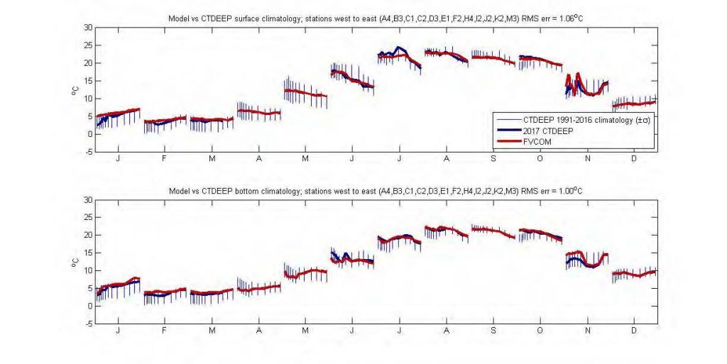
Plots by month showing surface (top panel) and bottom (bottom panel) temperature comparisons between model predictions (red lines) and monthly climatologies from 1993-2016 CTDEEP survey data (thin vertical blue bars, ±σ) and the 2017 CTDEEP surveys (thick blue lines). Within each month, the CTDEEP stations are plotted by longitude from west to east.